Detection of Copy Number Variation in Targeted Sequencing Samples
Hong Zheng / 2017-08-28
Introduction
There are two categories of methods for copy number variation (CNV) detection.
Based on read pair information
1) The paired-end mapping approach, in which mapped paired-reads whose distances are significantly different from the predetermined average insert size are used.
Tools: BreakDancer, VariationHunter, PEMer, etc.
2) The split read (SR) approach identifies read pairs in which one read from each pair is aligned to the reference genome uniquely while the other one fails to map or only partially maps to the genome. Those unmapped or partially mapped reads potentially provide accurate breaking points at the single base pair level for CNVs or structural variants.
Tools: Pindel, BreakSeq2, DellyBased on read depth (RD) information
With the accumulation of high-coverage sequencing data, RD-based methods have become a major approach to estimate CNV. The underlying hypothesis is that the read depth of a genomic region is correlated with the copy number of the region.
1) For whole-genome sequencing (WGS), a sliding window approach is adopted.
Tools: CNVnator, CNVnorm, cn.MOPS, cnvHMM, CNV-seq, JointSLMb, etc.
2) For whole-exome sequencing (WES), due to differing capture efficiency and non-continuous distributions of the reads, the methods used for WGS are not suitable. Several special methods have been developed for WES.
a) multiple samples as input. XHMM, CODEX, CoNIFER, ExoCNVTest
b) case-control samples as input. ExomeCNV, CONTRA, PropSeq, VarScan2
c) Others. ExomeDepth, CONDEX, SeqGene, Control-FREEC
The read pair-based methods rely heavily on the location of breakpoints, CNV size relative to insert size, and read length. Due to the discontinuation of genomic regions in exome/targeted sequencing, most CNV breakpoints could not be detected using these methods.
In contrast, RD-based methods are good for detection of CNVs in scarce genomic regions. Moreover, RD-based methods can detect large insertions and CNVs in complex genomic regions, which are difficult to detect using read pair-based methods.
For RD-based methods, instead of looking at a single sample one time, more and more tools utilize multiple samples to increase sensitivity and reduce false discovery.
In this demo, both the read pair-based and RD-based methods were deployed to investigate the CNVs in targeted sequencing data. The methods that have been used are emphasized in bold font in the text.
Results
Ground-truth 1000 Genome CNV data
########
#download
########
wget ftp://ftp.ncbi.nlm.nih.gov/pub/dbVar/data/Homo_sapiens/by_study/estd219_1000_Genomes_Consortium_Phase_3_Integrated_SV/vcf/estd219_1000_Genomes_Consortium_Phase_3_Integrated_SV.GRCh37.submitted.variant_call.germline.vcf.gz

########
#process
########
pre=estd219_1000_Genomes_Consortium_Phase_3_Integrated_SV.GRCh37.submitted.variant_call.germline
zcat $pre.vcf.gz | egrep -v '^#' | sed 's/;/\t/g' | grep -v CIPOS | awk 'OFS="\t"{print $1,$2,$13,$12,$10,$9}' | sed 's/END=//;s/SAMPLE=//;s/SVTYPE=//;s/CALLID=//' > $pre.preciseCNV.txt
zcat $pre.vcf.gz | egrep -v '^#' | sed 's/;/\t/g' | grep CIPOS | awk 'OFS="\t"{print $1,$2,$15,$12,$10,$9}' | sed 's/END=//;s/SAMPLE=//;s/SVTYPE=//;s/CALLID=//' > $pre.impreciseCNV.txt
cat $pre.preciseCNV.txt $pre.impreciseCNV.txt > $pre.CNV.txt
XHMM
XHMM takes multiple samples as input. The demo is based on targeted sequencing data of 105 genes in 118 samples.
1) Calculate depth of coverage from BAM files
Input:
- A list of BAM files, generated properly from the established pipeline for variant calling.
- The BED file of targeted regions in proper format. The chromosome names should match with the BAM files. The chromosome names and starting coordinates should be sorted. Redundant or overlapping regions should be merged (bedtools merge). The choice of regions in the BED file is fairly important, as it is the basic unit for coverage calculation and CNV calling.
Scripts:
run_DepthOfCoverage.sh:
work_dir=/home/zhengh/projects/CNV/105genes
target=105genespure
interval_file=/home/database/targetBed/$target.bed

/home/pipelines/DepthOfCoverage.sh \
       $work_dir/bam.list $interval_file $work_dir/QC $target \
       1> $work_dir/logs/$target.DepthOfCoverage.log 2>&1
DepthOfCoverage.sh:
bamlist=$1
interval_file=$2
QC_dir=$3
interval=$4

DIR="${BASH_SOURCE%/*}";if [[ ! -d "$DIR" ]]; then DIR="$PWD"; fi
source "$DIR/DATABASESandTOOLS.sh"

###-------Tutorial------------------------------------------------------------------------------------------------------
### http://gatkforums.broadinstitute.org/gatk/discussion/40/performing-sequence-coverage-analysis
###-------Tutorial------------------------------------------------------------------------------------------------------

###-------DepthOfCoverage-----------------------------------------------------------------------------------------------
echo "Goodluck! DepthOfCoverage started on `date`"

$java -Xmx8G -jar $gatk -T DepthOfCoverage \
        -I $bamlist \
        -R $ref_dir/human_g1k_v37_decoy.fasta \
	-L $interval_file \
        -o $QC_dir/$interval.bam.DP \
	--minBaseQuality 0 --minMappingQuality 20 \
        --start 1 --stop 5000 --nBins 200 \
        -dt BY_SAMPLE -dcov 5000 \
        --includeRefNSites --countType COUNT_FRAGMENTS \
	-geneList $ref_dir/hg19.geneTrack.refSeq

echo "Goodluck! DepthOfCoverage finished on `date`"
###-------DepthOfCoverage-----------------------------------------------------------------------------------------------
Output:
Target  total_coverage  average_coverage        HG00707_S2_total_cvg    HG00707_S2_mean_cvg     HG00707_S2_granular_Q1 HG00707_S2_granular_median      HG00707_S2_granular_Q3  HG00707_S2_%_above_15
1:17345334-17345466     662773  4983.26 12917   97.12   94      99      104     100.0
1:17349079-17349268     878128  4621.73 16233   85.44   78      87      97      100.0
1:17350434-17350584     499734  3309.50 9242    61.21   58      64      69      100.0
1:17354219-17354360     669584  4715.38 13648   96.11   90      96      105     100.0
1:17355074-17355252     1200155 6704.78 22278   124.46  109     129     146     100.0
1:17359524-17359658     849562  6293.05 15855   117.44  108     123     134     100.0
2) XHMM calling
2.1) Change data format, remove samples and target regions that do not fulfill coverage requirments, and mean-center the coveage.
a) The”chr” are added to chromosome names to facilitate plots.
b) Here the default thresholds for coverage are used.
target mean coverage: between 10 and 500
sample mean coverage: between 25 and 200
In this case, 17 samples and 15 targets are removed due to low coverage. They are found in files ending with “filtered_centered.RD.txt.filtered_targets.txt” and “filtered_centered.RD.txt.filtered_samples.txt”.
Importantly, if the experimental setup is expected to result in mean depths that deviate from these generic values, then these values need to be changed to reflect the dataset and only remove true outlier targets and samples. The default values work well for the current dataset.
c) Center each column of the matrix (RD.txt) so that the mean target value is 0 in preparation for PCA based normalization in the next step.
work_dir=/home/zhengh/projects/CNV/105genes
xhmm=/home/tools/XHMM/statgen-xhmm-cc14e528d909/xhmm
covdata=$work_dir/QC/105genespure.bam.DP.sample_interval_summary
pre=118bam.105genespure
ref=/home/database/b37/human_g1k_v37_decoy.fasta
target=105genespure
interval_file=/home/database/targetBed/$target.bed
param=/home/tools/XHMM/statgen-xhmm-cc14e528d909/params.txt
param_adjusted=/home/zhengh/projects/CNV/105genes/xhmm/params.txt

########
echo "change data format. Good luck."
########
less $covdata | sed '2,$s/^/chr/' > $work_dir/xhmm/$pre.DP.sample_interval_summary
$xhmm --mergeGATKdepths -o $work_dir/xhmm/$pre.RD.txt --GATKdepths $work_dir/xhmm/$pre.DP.sample_interval_summary

#######
echo "mean-centers the targets. Good luck."
#######
$xhmm --matrix -r $work_dir/xhmm/$pre.RD.txt --centerData --centerType target \
-o $work_dir/xhmm/$pre.filtered_centered.RD.txt \
--outputExcludedTargets $work_dir/xhmm/$pre.filtered_centered.RD.txt.filtered_targets.txt \
--outputExcludedSamples $work_dir/xhmm/$pre.filtered_centered.RD.txt.filtered_samples.txt \
--minTargetSize 10 --maxTargetSize 10000 \
--minMeanTargetRD 10 --maxMeanTargetRD 500 \
--minMeanSampleRD 25 --maxMeanSampleRD 200 \
--maxSdSampleRD 150
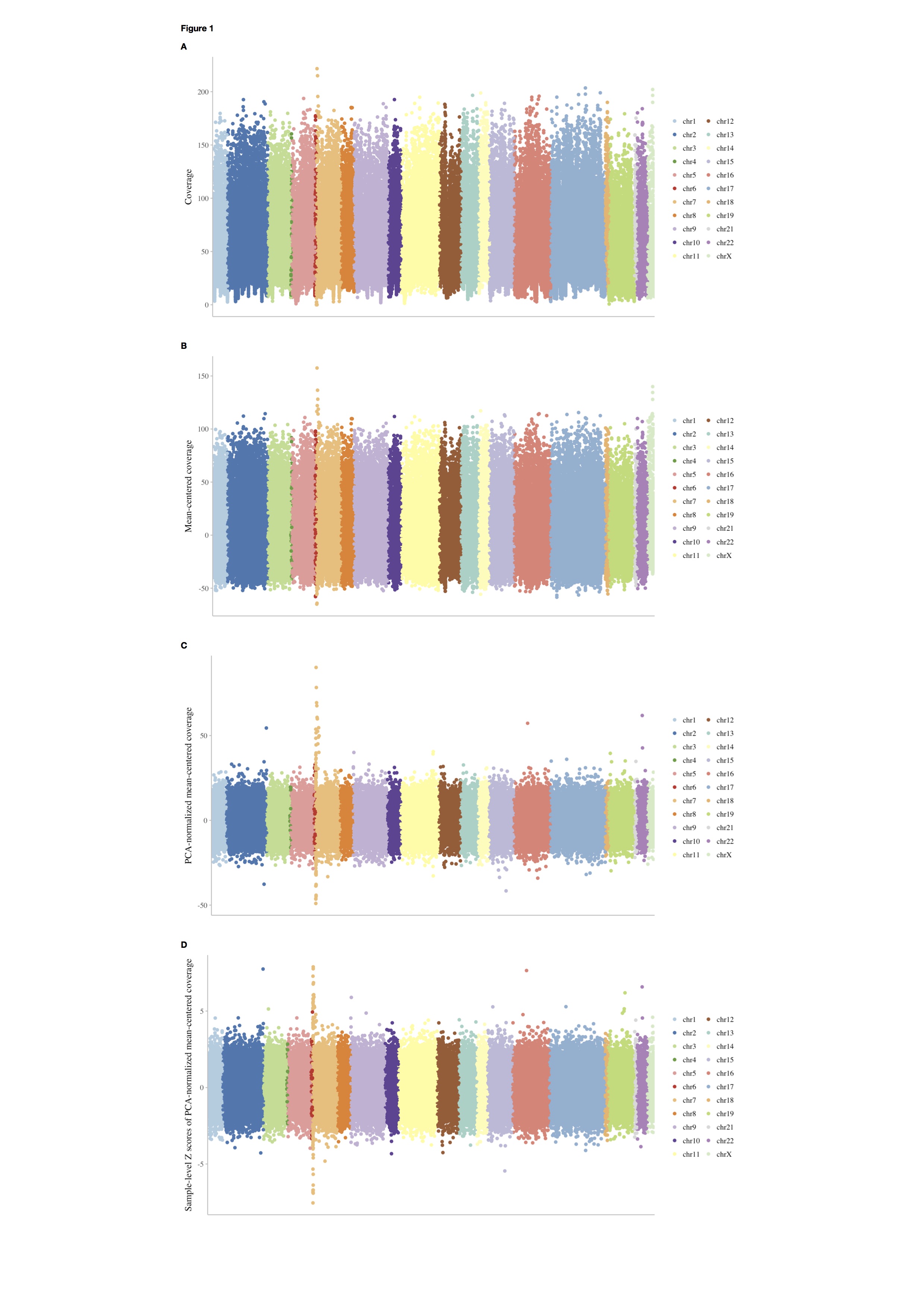
Raw coverage (RD.txt) and the output mean-centered coverage after filtering (filtered_centered.RD.txt) are shown in Figure 1A and 1B.
2.2) Run principal component analysis (PCA) on mean-centered data, and then normalizes the data using PCA information.
PCA analysis is used to determine the strongest independent ways (principal components) in which the data varies and remove the strongest signals that are driven by factors that do not reflect true CNV.
In this case, the first 2 PCs are removed from the datasets.
########
echo "Runs PCA on mean-centered data. Good luck."
#######
$xhmm --PCA -r $work_dir/xhmm/$pre.filtered_centered.RD.txt --PCAfiles $work_dir/xhmm/$pre.RD_PCA

#######
echo "Normalizes mean-centered data using PCA information. Good luck."
#######
$xhmm --normalize -r $work_dir/xhmm/$pre.filtered_centered.RD.txt --PCAfiles $work_dir/xhmm/$pre.RD_PCA \
--normalizeOutput $work_dir/xhmm/$pre.PCA_normalized.txt \
--PCnormalizeMethod PVE_mean --PVE_mean_factor 0.7
In the above codes, the first step outputs 3 files to be used in the next step:
DATA.RD_PCA.PC.txt: the data projected into the principal components
DATA.RD_PCA.PC_LOADINGS.txt: the loadings of the samples on the principal components
DATA.RD_PCA.PC_SD.txt: the variance of the input read depth data in each of the principal components
In the second step, the number of principal components to be removed is determined by the --PCnormalizeMethod PVE_mean --PVE_mean_factor 0.7 argument, which indicates that any principal component in which the data variance is greater than 0.7 times the mean variance over all components will be removed. This argument can be changed to retain additional components or remove more components for normalization.
The coverage after PCA normalization is shown in Figure 1C.
2.3) Z-score normalization and further filtering.
The PCA-normalized coverage data might still have some targets that have very high variance that may be reflective of failed normalization, thus, they are removed in this step. Note, however, that even after this filtering step, exon targets with very high variance in the original read depths still remain with relatively high (though attenuated) variance in depth after normalization, since large differences between samples and targets are by necessity maintained in order to preserve existing CNV signal as well. Then, for each sample, a z-score is calculated by centering relative to all target depths in that sample.
Next, the same targets and samples that are removed during the normalization process are also removed in the original dataset. This matrix will be used for annotation purposes in the subsequent CNV discovery steps.
#######
echo "Filters and z-score centers (by sample) the PCA-normalized data. Good luck."
#######
$xhmm --matrix -r $work_dir/xhmm/$pre.PCA_normalized.txt --centerData --centerType sample --zScoreData \
-o $work_dir/xhmm/$pre.PCA_normalized.filtered.sample_zscores.RD.txt \
--outputExcludedTargets $work_dir/xhmm/$pre.PCA_normalized.filtered.sample_zscores.RD.txt.filtered_targets.txt \
--outputExcludedSamples $work_dir/xhmm/$pre.PCA_normalized.filtered.sample_zscores.RD.txt.filtered_samples.txt \
--maxSdTargetRD 30

#######
echo "Filters original read-depth data to be the same as filtered, normalized data. Good luck."
#######
$xhmm --matrix -r $work_dir/xhmm/$pre.RD.txt \
--excludeTargets $work_dir/xhmm/$pre.filtered_centered.RD.txt.filtered_targets.txt \
--excludeTargets $work_dir/xhmm/$pre.PCA_normalized.filtered.sample_zscores.RD.txt.filtered_targets.txt \
--excludeSamples $work_dir/xhmm/$pre.filtered_centered.RD.txt.filtered_samples.txt \
--excludeSamples $work_dir/xhmm/$pre.PCA_normalized.filtered.sample_zscores.RD.txt.filtered_samples.txt \
-o $work_dir/xhmm/$pre.same_filtered.RD.txt
The coverage after Z score normalization is shown in Figure 1D.
2.4) Genotyping CNVs.
A hidden Markov model (HMM) with certain properties that were derived from a large-scale trio data set is applied in this step. The parameters, which determine the rate and length of the CNV called, are specified in params.txt (1e-8 6 70 -3 1.00 0 1.00 3 1.00)
The 9 values in this file correspond to quantities that respectively define the:
- Exome-wide CNV rate
- Mean number of targets in a CNV call
- Mean distance between targets within a CNV (in KB)
- Mean of DELETION z-score distribution
- Standard deviation of DELETION z-score distribution
- Mean of DIPLOID z-score distribution
- Standard deviation of DIPLOID z-score distribution
- Mean of DUPLICATION z-score distribution
- Standard deviation of DUPLICATION z-score distribution
These parameters are used in the HMM for CNV discovery and genotyping. They may need modification to suit the needs of particular project. For example, to increase the number of CNV calls, increase the first parameter from its default value of 1e-8, e.g., to 1e-7.
The parameters used for the current datasets are (1e-8 6 70 -3 1.1 0 0.9 3 1.1)
#######
echo "Discovers CNVs in normalized data. Good luck."
#######
$xhmm --discover -p $param_adjusted \
-r $work_dir/xhmm/$pre.PCA_normalized.filtered.sample_zscores.RD.txt -R $work_dir/xhmm/$pre.same_filtered.RD.txt \
-c $work_dir/xhmm/$pre.xcnv -a $work_dir/xhmm/$pre.aux_xcnv -s $work_dir/xhmm/$pre
Output file (.xcnv):
SAMPLE  CNV     INTERVAL        KB      CHR     MID_BP  TARGETS NUM_TARG        Q_EXACT Q_SOME  Q_NON_DIPLOID   Q_START Q_STOP  MEAN_RD MEAN_ORIG_RD
NA12889_S61     DUP     chr7:6017194-6018339    1.15    chr7    6017766 412..413        2       67      88      88      20      25      6.33    135.48
NA18873_S38     DUP     chr7:6017194-6018339    1.15    chr7    6017766 412..413        2       50      50      50      6       29      5.46    59.16
HG00451_S34     DUP     chr7:6012999-6048725    35.73   chr7    6030862 411..425        15      10      99      99      1       53      4.79    157.75
NA18609_S49     DUP     chr7:6017194-6018339    1.15    chr7    6017766 412..413        2       25      36      36      22      7       4.96    107.23
HG00692_S10     DEL     chr7:6012999-6022639    9.64    chr7    6017819 411..414        4       7       99      99      23      5       -4.84   16.56
HG01872_S48     DUP     chr22:29115357-29121386 6.03    chr22   29118371        1698..1700      3       14      70      70      14      8       4.52    136.17
HG00684_S13     DUP     chr7:6012999-6018339    5.34    chr7    6015669 411..413        3       5       99      99      5       21      5.10    79.65
NA18622_S55     DUP     chr2:233198528-233208282        9.76    chr2    233203405       212..218        7       30      99      99      14      50      3.72    76.54
NA18558_S39     DEL     chr15:80454562-80460700 6.14    chr15   80457631        1162..1164      3       35      39      39      4       27      -4.04   29.29
HG00629_S27     DEL     chr7:6012999-6018339    5.34    chr7    6015669 411..413        3       21      99      99      21      5       -5.13   12.96
NA18624_S59     DEL     chr7:6012999-6018339    5.34    chr7    6015669 411..413        3       3       99      99      3       7       -4.88   21.31
HG02522_S57     DUP     chr7:6012999-6018339    5.34    chr7    6015669 411..413        3       20      41      41      21      13      4.11    67.96
NA11995_S51     DEL     chr7:6012999-6018339    5.34    chr7    6015669 411..413        3       9       99      99      9       27      -5.21   0.15
NA07357_S45     DUP     chr19:45855446-45873862 18.42   chr19   45864654        1621..1643      23      5       99      99      10      5       3.03    51.15
NA18628_S59     DUP     chr7:6012999-6018339    5.34    chr7    6015669 411..413        3       9       37      37      9       8       3.96    38.32
HG00634_S26     DUP     chr16:23614761-23615012 0.25    chr16   23614886        1247..1247      1       30      30      30      30      23      7.65    155.58
NA18572_S44     DUP     chr9:271606-289600      18.00   chr9    280603  560..562        3       48      80      80      48      15      4.80    105.55
Each line is one CNV called in an individual. Column meaning:
- SAMPLE sample name in which CNV was called
- CNV type of copy number variation (DEL or DUP)
- INTERVAL genomic range of the called CNV
- KB length in kilobases of called CNV
- CHR chromosome name on which CNV falls
- MID_BP the midpoint of the CNV
- TARGETS the range of the target indices over which the CNV is called
- NUM_TARG # of exome targets of the CNV
- Q_EXACT Phred-scaled quality of the exact CNV event along the entire interval
- Q_SOME Phred-scaled quality of some CNV event in the interval
- Q_NON_DIPLOID Phred-scaled quality of not being diploid, i.e., DEL or DUP event in the interval
- Q_START Phred-scaled quality of “left” breakpoint of CNV
- Q_STOP Phred-scaled quality of ‘right” breakpoint of CNV
- MEAN_RD Mean normalized read depth (z-score) over interval
- MEAN_ORIG_RD Mean read depth (# of reads) over interval
3) Compare with ground truth
#######
echo "Get ground truth CNV from 1000G"
#######
CNV_1000G=../1000g/estd219_1000_Genomes_Consortium_Phase_3_Integrated_SV.GRCh37.submitted.variant_call.germline.CNV.txt
sed 's/_.*//' $pre.samplesID.filter  > 1000GsampleID.exclude # get the list of samples IDs to be excluded because of coverge issues
sed 's/_.*//' ../sampleID > 1000GsampleID # get the list of all samples IDs
less $pre.targetsID.filter | sed 's/:/\t/;s/-/\t/;s/chr//' |awk 'OFS="\t"{$2=$2-1;print $0}' | sort -k1,1n -k2,2n | subtractBed -a $interval_file -b - > $target.1000G.bed # get the target regions after removing regions with abnormal coverage

Extract.pl 1000GsampleID 1 $CNV_1000G 4  | Exclude.pl 1000GsampleID.exclude 1 - 4 > $pre.1000G.cnv.tmp # get CNVs in selected samples
intersectBed -a $pre.1000G.cnv.tmp -b $target.1000G.bed > $pre.1000G.cnv.tmpa # get CNVs in selected targets
./cnv.adjectmerge.pl $pre.1000G.cnv.tmpa | sort -k1,1n -k2,2n > $pre.1000G.cnv.txt # merge multiple record of the same CNV into one
cat 118bam.105genespure.1000G.cnv.txt
2       233200457       233208282       NA18622 DUP     DUP_gs_CNV_2_233200004_233214555_NA18622
7       6031568 6038922 HG00451 DUP     DUP_gs_CNV_7_6031005_6039619_HG00451
9       271605  289600  NA18572 DUP     DUP_gs_CNV_9_224074_289974_NA18572
15      80454561        80460700        NA18558 DEL     UW_VH_20565_NA18558
16      23614760        23615012        HG00634 DUP     DUP_gs_CNV_16_23608128_23616407_HG00634
19      45854860        45873862        NA07357 DUP     DUP_gs_CNV_19_45845933_45876990_NA07357
19      45854860        45873862        NA07357 DUP     DUP_uwash_chr19_45826405_45907191_NA07357
22      29115356        29121386        HG01872 DUP     DUP_gs_CNV_22_29114293_29125290_HG01872
Comparing XHMM results with ground truth, we can see that except the one region in chr7 (the region has high-variance in coverage), CNV calls in all other regions are concordant.
ExomeDepth
ExomeDepth runs in three steps.
- Calculate read depth across the datasets, which is similar to XHMM.
- Generate a panel of reference samples that are copy-number neutral.
- For each test sample, compare it against the panel of reference samples, and call CNVs.
Input:
BAM files, interval file, genome fasta file, reference sample IDs (multiple), test sample ID (single)
In the trial, 84 samples that fulfill the following criteria are chosen as reference samples:
- Do not have CNV event in 1000 Genome
- Do not have CNV event in XHMM results
- Sufficient read depth (Mean Sample RD: 25~200)
Scripts:
library(ExomeDepth)

#######
#echo "prepare input bam, bed, and genome fasta files"
#######
bedFile <- file.path("/home/database/targetBed", "105genespure.txt")
targets <- read.table(bedFile,head=T)
b37<-file.path("/home/database/b37","human_g1k_v37_decoy.fasta")
bamName <- list.files("/home/zhengh/projects/CNV/105genes/bam", pattern = '*.bam$')
bamFile <- file.path("/home/zhengh/projects/CNV/105genes/bam",bamName)

#######
#echo "get counts for target regions"
#######
TargetCount <- getBamCounts(bed.frame = targets,bam.files = bamFile,include.chr = FALSE,referenceFasta = b37)
TargetCount.df <- as(TargetCount[, colnames(TargetCount)], 'data.frame')

#######
#echo "prepare reference samples"
#######
sampleID.nocnv<-scan("/home/zhengh/projects/CNV/105genes/xhmm/sampleID.noCNV",quiet=T,what="character")
my.ref.samples <- paste0(sampleID.nocnv,".mapped.dedupped.realigned.recalled.bam")
my.reference.set <- as.matrix(TargetCount.df[, my.ref.samples])

#######
#echo "CNV calling per sample"
#######
sampleID<-scan("/home/zhengh/projects/CNV/105genes/ExomeDepth/samples",quiet=T,what="character")
for (Sample in sampleID){

my.test <- TargetCount.df[,paste0(Sample,".mapped.dedupped.realigned.recalled.bam")]
my.choice <- select.reference.set (test.counts = my.test,
        reference.counts = my.reference.set,
        bin.length = (TargetCount.df$end - TargetCount.df$start)/1000,
        n.bins.reduced = 10000)

my.matrix <- as.matrix( TargetCount.df[, my.choice$reference.choice, drop = FALSE])
my.reference.selected <- apply(X = my.matrix, MAR = 1, FUN = sum)

all.exons <- new('ExomeDepth',
        test = my.test,
        reference = my.reference.selected,
        formula = 'cbind(test, reference) ~ 1')

all.exons <- CallCNVs(x = all.exons,
        transition.probability = 10^-4,
        chromosome = TargetCount.df$space,
        start = TargetCount.df$start,
        end = TargetCount.df$end,
        name = TargetCount.df$names)

if(nrow(all.exons@CNV.calls)>0){
        output.file <- paste0(Sample,".cnv.txt")
        write.table(file = file.path("/home/zhengh/projects/CNV/105genes/ExomeDepth/out",output.file),x = cbind(Sample,all.exons@CNV.calls),row.names = FALSE,quote=F,sep="\t")
}
}
Output:
cat *.txt | egrep -v 'Sample' | sort -k8n |cut -f1,4,9
HG02522_S57     duplication     chrX:154002844-154004606
NA18622_S55     duplication     chr2:233198528-233208282
HG00451_S34     duplication     chr6:26092804-26094703
HG00451_S34     duplication     chr7:6012999-6048725
HG00629_S27     deletion        chr7:6012999-6018339
HG00684_S13     duplication     chr7:6017194-6018339
HG00692_S10     deletion        chr7:6012999-6018339
HG01872_S48     deletion        chr7:6012999-6013213
NA11995_S51     deletion        chr7:6012999-6018339
NA12889_S61     duplication     chr7:6017194-6018339
NA18609_S49     duplication     chr7:6017194-6018339
NA18624_S59     deletion        chr7:6012999-6018339
NA18873_S38     duplication     chr7:6017194-6018339
NA18572_S44     duplication     chr9:214926-289600
HG01872_S48     duplication     chr11:118955719-118955888
NA11995_S51     deletion        chr15:40493079-40493221
NA18558_S39     deletion        chr15:80454562-80460700
HG00634_S26     duplication     chr16:23614761-23615012
NA07357_S45     duplication     chr19:45855446-45873862
HG01872_S48     duplication     chr22:29115357-29121386
Similar to XHMM result, the region in chr7 is quite ambiguous and may not be trustable. Except for chr7 regions, ExomeDepth identifies all the other CNV events in the ground truth 1000 Genome data. Besides, ExomeDepth also detects extra CNVs not present in 1000 Genome and XHMM results, and the accuracy remains to be evaluated.
CODEX
CODEX takes multiple samples as input.
Input:
BAM files, bed file, and sample IDs
Script:
library(CODEX2)
setwd("/home/zhengh/projects/CNV/105genes/CODEX")

######################################################
######################################################
####                                              ####
####          get coverage, gc, mapp              ####
####                                              ####
######################################################
######################################################

bamName <- list.files("/home/zhengh/projects/CNV/105genes/bam", pattern = '*.bam$')
bamFile <- file.path("/home/zhengh/projects/CNV/105genes/bam",bamName)
sampname <- as.matrix(read.table(file.path("/home/zhengh/projects/CNV/105genes", "sampleID")))
bedFile <- file.path("/home/database/targetBed", "105genes.primary_targets.bed")
projectname<-"CNV_prenetics"

chr=1
# get bam directories, read in bed file, get sample names
bambedObj=getbambed(bamdir=bamFile,
                    bedFile=bedFile,
                    sampname=sampname,
                    projectname=projectname,chr)
bamdir=bambedObj$bamdir; sampname=bambedObj$sampname; ref=bambedObj$ref; projectname=bambedObj$projectname;chr=bambedObj$chr
# get raw depth of coverage
coverageObj=getcoverage(bambedObj,mapqthres=20)
Y=coverageObj$Y; readlength=coverageObj$readlength
# get gc content
gc=getgc(chr,ref)
# get mappability
mapp=getmapp(chr,ref)

ref.all=bambedObj$ref
Y.all=coverageObj$Y
gc.all=gc
mapp.all=mapp
chr.all=rep(chr,length=length(mapp))

targ.chr <- unique(as.matrix(read.table(bedFile, sep = "\t")[,1]))

for(chr in 2:23){
  if(chr==23){chr='X'}
  if(!is.element(chr,targ.chr)) next
  # get bam directories, read in bed file, get sample names
  bambedObj=getbambed(bamdir=bamdir,
                      bedFile=bedFile,
                      sampname=sampname,
                      projectname=projectname,chr)
  bamdir=bambedObj$bamdir; sampname=bambedObj$sampname; ref=bambedObj$ref; projectname=bambedObj$projectname;chr=bambedObj$chr
  # get raw depth of coverage
  coverageObj=getcoverage(bambedObj,mapqthres=20)
  Y=coverageObj$Y; readlength=coverageObj$readlength
  # get gc content
  gc=getgc(chr,ref)
  # get mappability
  mapp=getmapp(chr,ref)

  ref.all=c(ref.all,bambedObj$ref)
  Y.all=rbind(Y.all,coverageObj$Y)
  gc.all=c(gc.all,gc)
  mapp.all=c(mapp.all,mapp)
  chr.all=c(chr.all,rep(chr,length=length(mapp)))
}

save.image(file=paste(projectname,'_','coverage','.rda',sep=''))

######################################################
######################################################
####                                              ####
####                   normalize                  ####
####                                              ####
######################################################
######################################################

load(paste(projectname,'_coverage.rda',sep=''))

ref.all
length(chr.all)
dim(Y.all)
length(gc.all)
length(mapp.all)

gene.all=as.matrix(read.table('/home/database/targetBed/105genes.capture_targets.bed',head=F,sep='\t')[,4])
length(gene.all)

Y=Y.all
ref=ref.all
gc=gc.all
mapp=mapp.all
gene=gene.all

cov_thres1 =  20
cov_thres2 =  500
sample_median_thres = 25
qcObj=qc(Y,sampname,chr,ref,mapp,gc,cov_thresh=c(cov_thres1,cov_thres2),length_thresh=c(20,2000),mapp_thresh=0.9,gc_thresh=c(20,80))
Y_qc=qcObj$Y_qc; sampname_qc=qcObj$sampname_qc; gc_qc=qcObj$gc_qc; mapp_qc=qcObj$mapp_qc; ref_qc=qcObj$ref_qc ; qcmat=qcObj$qcmat
dim(Y_qc)
length(gc_qc)
length(mapp_qc)
gene_qc=gene[which(as.logical(qcmat[,4])==TRUE)]
chr_qc=chr.all[which(as.logical(qcmat[,4])==TRUE)]
length(gene_qc)
length(sampname_qc)

sampfilter=apply(Y_qc,2,median)>=sample_median_thres
sampname_qc=sampname_qc[sampfilter]
Y_qc=Y_qc[,sampfilter]
rm(qcObj)

normObj <- normalize(Y_qc, gc_qc, K = 1:10)
Yhat <- normObj$Yhat; AIC <- normObj$AIC; BIC <- normObj$BIC ;RSS <- normObj$RSS; K <- normObj$K

save.image(file=paste(projectname,'_','normalize','.rda',sep=''))

######################################################
######################################################
####                                              ####
####                    segment                   ####
####                                              ####
######################################################
######################################################

load(paste(projectname,'_normalize.rda',sep=''))

choiceofK(AIC,BIC,RSS,K,filename=paste(projectname,'_choiceofK','.pdf',sep=''))

dim(Y_qc)
length(ref_qc)
length(sampname_qc)
dim(Yhat[[2]])
length(chr_qc)

#plot(K, RSS, type = "b", xlab = "Number of latent variables")
#plot(K, AIC, type = "b", xlab = "Number of latent variables")
#plot(K, BIC, type = "b", xlab = "Number of latent variables")


optK=which.max(BIC)
optK=1
source('/home/zhengh/projects/CNV/105genes/CODEX/segment_targeted.R')
finalcall=matrix(ncol=14)
colnames(finalcall)=c('sample_name','chr','gene','cnv',
                      'st_bp','ed_bp','length_kb',
                      'st_exon','ed_exon','raw_cov',
                      'norm_cov','copy_no','lratio',
                      'mBIC')

for(genei in unique(gene_qc)){
  cat('Segmenting gene',genei,'\n')
  geneindex=which(gene_qc==genei)
  yi=Y_qc[geneindex,]
  yhati=Yhat[[optK]][geneindex,]
  refi=ref_qc[geneindex]
  chri=chr_qc[geneindex][1]
  finalcalli=segment_targeted(yi, yhati, sampname_qc, refi, genei, chri, lmax=length(geneindex), mode='fraction')
  finalcall=rbind(finalcall,finalcalli)
}

finalcall=finalcall[-1,]
cn=(as.numeric(as.matrix(finalcall[,'copy_no'])))
cn.filter=(cn<=1.7)|(cn>=2.3)
finalcall=finalcall[cn.filter,]

length_exon=as.numeric(finalcall[,'ed_exon'])-as.numeric(finalcall[,'st_exon'])+1
finalcall=cbind(finalcall[,1:7],length_exon,finalcall[,10:14])

write.table(finalcall, file = paste( projectname,'_', optK, '_CODEX_frac.txt',
                                     sep=''), sep='\t', quote=F, row.names=F)
save.image(file=paste(projectname,'_','finalcall','.rda',sep=''))
Output:
There are two many CNV calls and false discovery rate is very high.
Read pair-based methods
Several methods based on read pairs, including BreakDancer, Pindel, and BreakSeq2 have been utilized to examine the datasets. As expected, these methods don’t perform well for targeted sequencing datasets. Due to that fact that most breakpoints do not fall into exon regions, these methods can hardly identify true CNVs, and the results are mainly false positives. Therefore, the detailed scripts and results are not shown here. They can be found in /home/zhengh/projects/CNV/105genes/.
Other methods
Besides XHMM, ExomeDepth, CODEX, and several read-pair based methods, two other methods were also tested, but with no meaningful outputs.
- CNVnator. This tool is only suitable for whole genome sequencing.
- CoNIFER. This tool is only suitable for whole exome sequencing or genome sequencing. Targeted sequencing has too few targets.
Conclusion
To identify CNVs from targeted sequencing data, RD-based methods perform better than read pair-based methods. Among the RD-based methods, XHMM and ExomeDepth are both good at CNV detection utilizing a population of samples.
- XHMM works with multiple samples in each stage of the workflow.
- ExomeDepth also need multiple samples at the first stage to build a panel of reference. After the reference panel is ready, ExomeDepth can take in single sample each time, compare it with reference panel, and output CNV calls in the single sample.
- The results of XHMM and ExomeDepth are highly consistent and they both can identify CNVs in 1000 Genome ground truth dataset, except for a few problematic regions. In future workflow, these two methods can be combined to get a more confident CNV callset.
Several aspects need to be paid attention to:
- Sufficient sample size and number of targeted region are needed to accurately model the read depths and detect CNVs.
- The RD-based CNV methods, including XHMM and ExomeDepth , depend on a set of normal samples (without CNV changes) in the datasets to serve as baseline for CNV calling. For example, if all the samples in the datasets have deletions in a specific region, these methods will classify it as systematic problem (failure to capture, mapping problem etc.) and will not output the region as deletion event.
- Fine tuning of the parameters/choices of samples is needed in future workflow to achieve high accuracy.